

Next: 3.3.10 Concave Up Functions
Up: 3.3 Linear Interval Arithmetic
Previous: 3.3.8 Example with a Linear
Consider the floor function,  ,
which is a piecewise constant function.
We previously stated that
another possibility is to let
With either sectioning, the function is seen to be piecewise linear,
and is monotonically increasing:
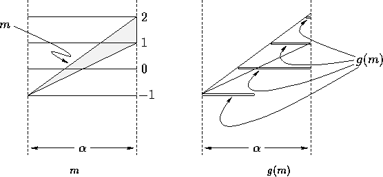
Consider the following diagram:
This type of diagram will be used throughout this section.
The light grey region will often represent g(m),
as it does in the rightmost diagram:
In the leftmost diagram, the region represents
m; the two diagrams together illustrate how  was determined.
The evaluation of  ,
,
proceeds as follows, using the first sectioning:
with
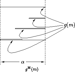
Perusal of the following figure may ease the comprehension
of the preceding evaluation.
The grey region represents g(m), while  is displayed as the upper and lower solid lines.
The evaluation of  ,
,
proceeds as follows, using the second sectioning:
with
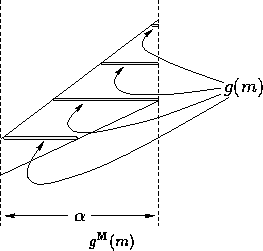
The following figure graphically illustrates portions of the
preceding evaluation.
Which of the two methods is used depends on the values
of
The same method need not be used for both bounds.
With a reasonable choice of  ,
an optimal bound is easily computed.


Next: 3.3.10 Concave Up Functions
Up: 3.3 Linear Interval Arithmetic
Previous: 3.3.8 Example with a Linear
![]() ,
which is a piecewise constant function.
We previously stated that
,
which is a piecewise constant function.
We previously stated that
![]()
![]()
![]()

![]()
![]() ,
,
![]()

![]()
![]()

![]() ,
,
![]()

![]()
![]()

![]()